Pandas模块
Pandas 是基于 NumPy 的一种数据处理工具,该工具为了解决数据分析任务而创建。Pandas 纳入了大量库和一些标准的数据模型,提供了高效地操作大型数据集所需的函数和方法。
Pandas 的数据结构:Pandas 主要有 Series(一维数组),DataFrame(二维数组),Panel(三维数组),Panel4D(四维数组),PanelND(更多维数组)等数据结构。其中 Series 和 DataFrame 应用的最为广泛。
Pandas 的数据处理功能十分强大,本文只对常用的功能做一个梳理,帮助快速熟悉。
首先,你需要将其引入:
import pandas as pd
import numpy as np
生成数据
Series
# 基于列表创建,或者 numpy 列表都可以
s = pd . Series ([ 1 , 3 , 5 , np . nan , 6 , 8 ])
# 指定索引
s2 = pd . Series ([ 4 , 7 , - 5 , 3 ], index = [ 'd' , 'b' , 'a' , 'c' ])
# 通过字典创建
sdata = { 'Ohio' : 35000 , 'Texas' : 71000 , 'Oregon' : 16000 , 'Utah' : 5000 }
s3 = pd . Series ( sdata )
# 通过字典创建时,你可以指定 index 的顺序
states = [ 'California' , 'Ohio' , 'Oregon' , 'Texas' ]
s4 = pd . Series ( sdata , index = states )
你可以把 Series 看做是一个定长的有序字典。可以使用 in 来判断一个索引是否存在:
Series 本身及其索引都有一个 name 属性,该属性与 pandas 其他的关键功能关系非常密切:
In [ 4 ]: s4 . name = 'population'
In [ 4 ]: s4 . index . name = 'state'
In [ 5 ]: s4
Out [ 5 ]:
state
California NaN
Ohio 35000.0
Oregon 16000.0
Texas 71000.0
Name : population , dtype : float64
Series 的索引可以通过赋值的方式就地修改:
In [ 6 ]: s4 . index = [ "A" , "B" , "C" , "D" ]
In [ 7 ]: s4
Out [ 7 ]:
A NaN
B 35000.0
C 16000.0
D 71000.0
Name : population , dtype : float64
Note
虽然可以对 Series 的 index 进行修改,但是 index 对象本身是不可变的,这意味着无法进行以下操作:
idx = s4 . index
idx [ 1 ] = 'd' #TypeError
这种不可变的特性,使得 Index 对象可以在多个数据结构之间安全共享。Index 对象类似于一个固定大小的集合,但是与传统集合不同的是,它可以包含重复元素,选择重复的标签会显示所有的结果。
Index 的一些方法和属性:
方法
说明
append
连接另一个Index对象,产生一个新的 index
difference
计算差集,并得到一个Index
intersection
计算交集
union
计算并集
isin
计算一个指示各值是否都包含在参数集合中的布尔型数组
delete
删除索引 i 处的元素,并得到新的 Index
drop
删除传入的值,并得到新的 Index
insert
将元素插入到索引 i 处,并得到新的 Index
is_monotonic
当各元素均大于等于前一个元素时,返回 True
is_unique
当 Index 没有重复值时,返回 True
unique
计算 Index 中没有重复值的数组
DataFrame
DataFrame 既有行索引,又有列索引,它可以看做是由 Series 组成的字典。
In [ 1 ]: df = pd . DataFrame ({ 'A' : 1. ,
... : 'B' : pd . Timestamp ( '20130102' ),
... : 'C' : pd . Series ( 1 , index = list ( range ( 4 )), dtype = 'float32' ),
... : 'D' : np . array ([ 3 ] * 4 , dtype = 'int32' ),
... : 'E' : pd . Categorical ([ "test" , "train" , "test" , "train" ]),
... : 'F' : 'foo' })
In [ 2 ]: df
Out [ 2 ]:
A B C D E F
0 1.0 2013 - 01 - 02 1.0 3 test foo
1 1.0 2013 - 01 - 02 1.0 3 train foo
2 1.0 2013 - 01 - 02 1.0 3 test foo
3 1.0 2013 - 01 - 02 1.0 3 train foo
你也可以将一个二维数组直接传入 DataFrame,同时传入 columns 数组表示列索引。
In [ 7 ]: data = [[ 2 , 2 , 2 ], [ 3 , 3 , 3 ]]
In [ 8 ]: df = pd . DataFrame ( data , columns = [ 'A' , 'B' , 'C' ])
In [ 9 ]: df
Out [ 9 ]:
A B C
0 2 2 2
1 3 3 3
还有一种方式是嵌套字典,外层字典的键值作为列,内层键则作为行索引:
In [ 2 ]: pop = { 'Nevada' : { 2001 : 2.4 , 2002 : 2.9 }, 'Ohio' : { 2000 : 1.5 , 2001 : 1.7 , 2002 : 3.6 }}
In [ 3 ]: df = pd . DataFrame ( pop )
In [ 4 ]: df
Out [ 4 ]:
Nevada Ohio
2001 2.4 1.7
2002 2.9 3.6
2000 NaN 1.5
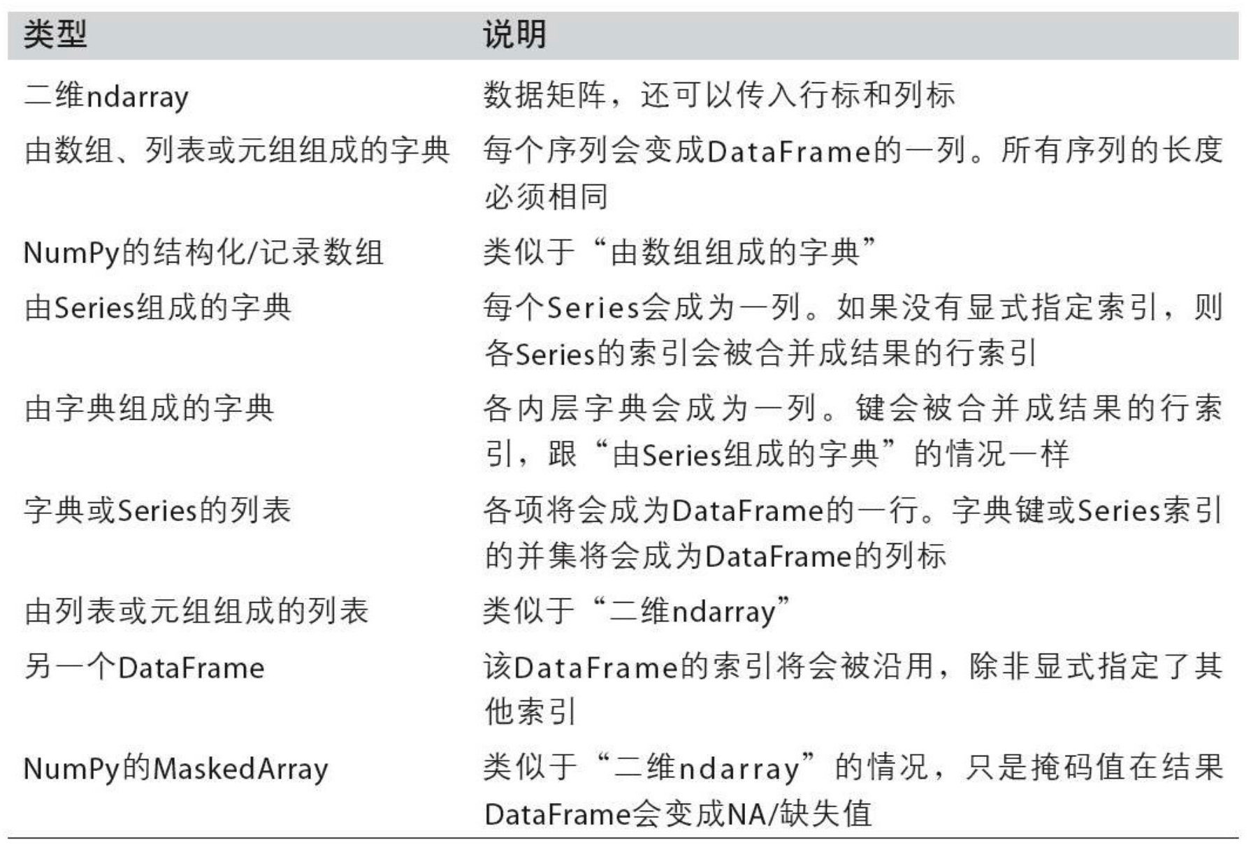
可以传给 DataFrame 构造器的数据如下表所示:
最后,你可以给 df.index.name 和 df.columns.name 设置名称,像 Series 一样。
查看数据
Note
注意,以下的大多数方法都是 DataFrame 的类方法,通过对象 df 来调用。只要少数方法是 pandas 的顶层方法,通过 pd 来调用。
并且,大多数的 df 方法都不会修改元数据对象,而是返回一个新的数据对象。这样做是为了保护元数据不被轻易修改。
df.head() 和 df.tail() 可以分别查看头部和尾部数据。
df.index 和 df.columns 可以分别查看索引和列名
df.to_numpy() 可以输出一个 numpy 数据类型。
因为 df 中可以存储不同类型的数据,如果这种 df 转成 numpy 的话,会自动变为 object 类型。如果 df 中存放的是基本的单一类型,转换会更快。
df.describe() 可以看查看摘要信息,包括每个列的统计信息。
df.T 可以将其转置
df.sort_values(by='B') 可以指定 df 按照某一列排序
df.sort_index(axis=1, ascending=False) 表示按轴降序排序。axis=1 表示对于每一行内的数据,将其按照列索引降序排列。
选择数据
Note
pandas 选择数据的方法有很多,都很方便。在正式生产环境中推荐使用 .at, iat, .loc, iloc 等优化后的方法。
Series
In [ 1 ]: s = pd . Series ([ 4 , 7 , - 5 , 3 ], index = [ 'd' , 'b' , 'a' , 'c' ])
In [ 2 ]: s
Out [ 2 ]:
d 4
b 7
a - 5
c 3
dtype : int64
对于 s 这样一个 Series,你可以通过 s.at['a'] 或者 s.loc['a'] 来访问 index 为 \(a\) 的元素,而它对应的下标是 2,因此也可以通过 s.iat[2] 或者 s.iloc[2] 来访问。
除此之外,你可以通过索引列表,批量访问多个元素:
In [ 3 ]: s [[ 'a' , 'b' , 'c' ]]
Out [ 3 ]:
a - 5
b 7
c 3
dtype : int64
又或者通过 Python 的切片:
In [ 4 ]: s [ 1 :]
Out [ 4 ]:
b 7
a - 5
c 3
dtype : int64
还有更厉害的是,通过布尔索引,返回 s 中所有大于 0 的元素:
In [ 6 ]: s [ s > 0 ]
Out [ 6 ]:
d 4
b 7
c 3
dtype : int64
DataFrame
Pandas 的每一个列是一个 Series,可以通过类似字典的方式去访问:
In [ 24 ]: data = { 'state' : [ 'Ohio' , 'Ohio' , 'Ohio' , 'Nevada' , 'Nevada' , 'Nevada' ], 'year' : [ 2000 , 2001 , 2002 , 2001 , 2002 , 2003 ], 'pop' : [ 1.5 , 1.7 , 3.6 , 2.4 , 2.9 , 3.2 ]}
In [ 25 ]: df = pd . DataFrame ( data )
In [ 26 ]: df
Out [ 26 ]:
state year pop
0 Ohio 2000 1.5
1 Ohio 2001 1.7
2 Ohio 2002 3.6
3 Nevada 2001 2.4
4 Nevada 2002 2.9
5 Nevada 2003 3.2
In [ 27 ]: df [ 'state' ]
Out [ 27 ]:
0 Ohio
1 Ohio
2 Ohio
3 Nevada
4 Nevada
5 Nevada
Name : state , dtype : object
但是如果要访问行,需要使用 loc 和 iloc
In [ 45 ]: df . loc [ 0 ]
Out [ 45 ]:
state Ohio
year 2000
pop 1.5
Name : 0 , dtype : object
In [ 50 ]: df . loc [ 0 , 'state' : 'year' ]
Out [ 50 ]:
state Ohio
year 2000
Name : 0 , dtype : object
In [ 51 ]: df . iloc [ 0 , 0 : 2 ]
Out [ 51 ]:
state Ohio
year 2000
Name : 0 , dtype : object
In [ 52 ]: df . iloc [ 0 , [ 0 , 1 ]]
Out [ 52 ]:
state Ohio
year 2000
Name : 0 , dtype : object
loc 和 iloc 的区别就是能否通过标签来访问,iloc 只能通过数字下标来访问。他们都支持切片的访问方法。
at 和 iat 只能访问单个元素,例如 df.at[0, 'state'],df.iat[0, 0]。
Info
布尔索引是一个非常好用的功能
In [ 54 ]: df
Out [ 54 ]:
state year pop
0 Ohio 2000 1.5
1 Ohio 2001 1.7
2 Ohio 2002 3.6
3 Nevada 2001 2.4
4 Nevada 2002 2.9
5 Nevada 2003 3.2
In [ 55 ]: df [ df [ 'year' ] > 2001 ]
Out [ 55 ]:
state year pop
2 Ohio 2002 3.6
4 Nevada 2002 2.9
5 Nevada 2003 3.2
In [ 56 ]: df [ df [ 'state' ] . isin ([ 'Ohio' ])]
Out [ 56 ]:
state year pop
0 Ohio 2000 1.5
1 Ohio 2001 1.7
2 Ohio 2002 3.6
如果遇到需要多个条件筛选时,可以用 &,|,~ 等将他们链接起来。
赋值
对于 Pandas 对象 df:
df['E'] = s,其中 s 是 Series 对象,Index 会自动对齐(相当于 df 与 s 根据 index 做 left join)。df.at[0, 'A'] = 0,按照标签赋值。df.iat[0, 1] = 0,按位置赋值。df.loc[:, 'D'] = np.array([5] * len(df)), 按 numpy 数组赋值。df[df > 0] = -df,用 where 条件赋值。
缺失值
Pandas 使用 np.nan 表示缺失值。计算时,默认不包含空值。通过 reindex,df 可以在副本上更改、添加、删除指定轴的索引。
df.dropna(how = 'any'),删除所有含缺失值的行,返回副本。df.fillna(value = 5),填充缺失值,返回副本。pd.isna(df) 或者 df.isna(),返回 nan 值的布尔掩码。
运算
一般情况下,运算时排除缺失值。
df.mean() 各列的平均值,df.mean(1) 各行的平均值
时间序列
date_range 可以很方便的生成本地时间序列,resample 可以根据指定频率聚合数据。
In [ 1 ]: rng = pd . date_range ( '1/1/2012' , periods = 100 , freq = 'S' )
In [ 2 ]: ts = pd . Series ( np . random . randint ( 0 , 500 , len ( rng )), index = rng )
In [ 3 ]: ts . resample ( '1Min' ) . sum ()
Out [ 3 ]:
2012 - 01 - 01 00 : 00 : 00 15439
2012 - 01 - 01 00 : 01 : 00 9327
Freq : T , dtype : int64
时区表示:
In [ 4 ]: rng = pd . date_range ( '3/6/2022 00:00:00' , periods = 5 , freq = 'D' )
In [ 5 ]: ts = pd . Series ( np . random . randn ( len ( rng )), rng )
In [ 6 ]: ts_utc = ts . tz_localize ( 'UTC' )
In [ 7 ]: ts_utc
Out [ 7 ]:
2022 - 03 - 06 00 : 00 : 00 + 00 : 00 1.185089
2022 - 03 - 07 00 : 00 : 00 + 00 : 00 - 0.537285
2022 - 03 - 08 00 : 00 : 00 + 00 : 00 0.802029
2022 - 03 - 09 00 : 00 : 00 + 00 : 00 - 0.047596
2022 - 03 - 10 00 : 00 : 00 + 00 : 00 - 0.646866
Freq : D , dtype : float64
转换成其他时区:
In [ 8 ]: ts_utc . tz_convert ( 'US/Eastern' )
Out [ 8 ]:
2012 - 03 - 05 19 : 00 : 00 - 05 : 00 0.464000
2012 - 03 - 06 19 : 00 : 00 - 05 : 00 0.227371
2012 - 03 - 07 19 : 00 : 00 - 05 : 00 - 0.496922
2012 - 03 - 08 19 : 00 : 00 - 05 : 00 0.306389
2012 - 03 - 09 19 : 00 : 00 - 05 : 00 - 2.290613
Freq : D , dtype : float64
基础部分
# 查看版本
print ( pd . __version__ )
Series
# 创建 Series
## 1. 从列表创建
arr = [ 0 , 1 , 2 , 3 , 4 ]
s1 = pd . Series ( arr ) # 如果不指定索引,则默认从 0 开始
## 2. 从 Ndarray 创建
n = np . random . randn ( 5 ) # 创建一个随机 Ndarray 数组
index = [ 'a' , 'b' , 'c' , 'd' , 'e' ]
s2 = pd . Series ( n , index = index ) # 指定 index
## 3. 从字典创建 Series
d = { 'a' : 1 , 'b' : 2 , 'c' : 3 , 'd' : 4 , 'e' : 5 } # 定义示例字典
s3 = pd . Series ( d )
# Series 基本操作
## 1. 修改索引
s1 . index = [ 'A' , 'B' , 'C' , 'D' , 'E' ]
## 2. 纵向拼接
s4 = s3 . append ( s1 )
## 3. 指定索引删除元素
s4 = s4 . drop ( 'e' )
## 4. 指定索引修改元素
s4 [ 'A' ] = 6
## 5. 切片操作
s4 [: 3 ]
# Series 运算
## 以下都是按照索引对应计算,如果不存在则填充为 NaN
s4 . add ( s3 )
s4 . sub ( s3 )
s4 . mul ( s3 )
s4 . div ( s3 )
s4 . median ()
s4 . sum ()
s4 . max ()
s4 . min ()
DataFrame
# 创建 DataFrame 数据类型
## 1. 通过 numpy 数组创建
dates = pd . date_range ( 'today' , periods = 6 )
num_arr = np . random . randn ( 6 , 4 )
columns = [ 'A' , 'B' , 'C' , 'D' ]
df1 = pd . DataFrame ( num_arr , index = dates , columns = columns )
## 2. 通过字典数组创建 DataFrame,字典的 key 将作为列,value 长度必须相同
data = { 'animal' : [ 'cat' , 'cat' , 'snake' , 'dog' , 'dog' , 'cat' , 'snake' , 'cat' , 'dog' , 'dog' ],
'age' : [ 2.5 , 3 , 0.5 , np . nan , 5 , 2 , 4.5 , np . nan , 7 , 3 ],
'visits' : [ 1 , 3 , 2 , 3 , 2 , 3 , 1 , 1 , 2 , 1 ],
'priority' : [ 'yes' , 'yes' , 'no' , 'yes' , 'no' , 'no' , 'no' , 'yes' , 'no' , 'no' ]}
labels = [ 'a' , 'b' , 'c' , 'd' , 'e' , 'f' , 'g' , 'h' , 'i' , 'j' ]
df2 = pd . DataFrame ( data , index = labels )
## 查看数据类型
df2 . dtypes
# DataFrame 基本操作
## 1. 查看前 5 行
df2 . head ()
## 2. 查看后 3 行
df2 . tail ( 3 )
## 3. 查看 index
df2 . index
## 4. 查看 columns
df2 . columns
## 5. 查看 dataframe 的数值
df2 . values
## 6. 查看统计数据
df2 . describe ()
## 7. 转置
df2 . T
## 8. 对 DataFrame 进行按列排序
df2 . sort_values ( by = 'age' )
## 9. 对 DataFrame 数据切片
df2 [ 1 : 3 ]
## 10. 通过便签查询(单列)
df2 [ 'age' ]
df2 . age
df2 [[ 'age' , 'animal' ]]
## 11. 通过位置查询
df2 . iloc [ 1 : 3 ]
## 12. 副本拷贝
df3 = df2 . copy ()
## 13. 判断 DataFrame 元素是否为空
df3 . isnull ()
## 14. 添加列数据
num = pd . Series ([ 0 , 1 , 2 , 3 , 4 , 5 , 6 , 7 , 8 , 9 ], index = df2 . index )
df3 [ 'No.' ] = num
## 15. 根据下标值进行更改
df3 . iat [ 1 , 1 ] = 2
## 16. 根据标签对数据进行修改
df3 . loc [ 'f' , 'age' ] = 1.5
## 17. 求平均值
df3 . mean ()
## 18. 对任意列做求和操作
df3 [ 'visits' ] . sum ()
字符串操作
## 将字符串转换为小写字母
string = pd . Series ([ 'A' , 'B' , 'C' , 'Aaba' , 'Baca' ,
np . nan , 'CABA' , 'dog' , 'cat' ])
print ( string )
string . str . lower ()
## 将字符串转换为大写字母
string . str . upper ()
DataFrame缺失值操作
## 对缺失值进行填充
df4 = df3 . copy ()
df4 . fillna ( value = 3 )
## 删除存在缺失值的行
df5 = df3 . copy ()
df5 . dropna ( how = 'any' )
## DataFrame 按指定列对齐,类似于 join 操作
left = pd . DataFrame ({ 'key' : [ 'foo1' , 'foo2' ], 'one' : [ 1 , 2 ]})
right = pd . DataFrame ({ 'key' : [ 'foo2' , 'foo3' ], 'two' : [ 4 , 5 ]})
# 按照 key 列对齐连接,只存在 foo2 相同,所以最后变成一行
pd . merge ( left , right , on = 'key' )
DataFrame 文件操作
## csv 文件写入
df3 . to_csv ( 'animal.csv' )
## csv 读入
df_animal = pd . read_csv ( 'animal.csv' )
## excel 写入
df3 . to_excel ( 'animal.xlsx' , sheet_name = 'Sheet1' )
## excel 读入
pd . read_excel ( 'animal.xlsx' , 'Sheet1' , index_col = None , na_values = [ 'NA' ])
进阶部分
时间序列索引
## 建立一个以 2018 年每一天为索引,值为随机数的 Series
dti = pd . date_range ( start = '2018-01-01' , end = '2018-12-31' , freq = 'D' )
s = pd . Series ( np . random . rand ( len ( dti )), index = dti )
## 统计 s 中每一个周三对应值的和
s [ s . index . weekday == 2 ] . sum ()
## 统计 s 中每个月的平均值
s . resample ( 'M' ) . mean ()
## 将 Series 中的时间进行转换(秒转分钟)
s = pd . date_range ( 'today' , periods = 100 , freq = 'S' )
ts = pd . Series ( np . random . randint ( 0 , 500 , len ( s )), index = s )
ts . resample ( 'Min' ) . sum ()
## UTC 世界时间标准
s = pd . date_range ( 'today' , periods = 1 , freq = 'D' )
ts = pd . Series ( np . random . randn ( len ( s )), s )
ts_utc = ts . tz_localize ( 'UTC' )
## 转为上海所在时区
ts_utc . tz_convert ( 'Asia/Shanghai' )
## 不同时间表示方式的转换
rng = pd . date_range ( '1/1/2018' , periods = 5 , freq = 'M' )
ts = pd . Series ( np . random . randn ( len ( rng )), index = rng )
ps = ts . to_period ()
ps . to_timestamp ()
Series 多重索引
## 创建多重索引 Series
letters = [ 'A' , 'B' , 'C' ]
numbers = list ( range ( 10 ))
mi = pd . MultiIndex . from_product ([ letters , numbers ])
s = pd . Series ( np . random . rand ( 30 ), index = mi )
## 多重索引 Series 查询
s . loc [:, [ 1 , 3 , 6 ]]
## 多重索引 Series 切片
s . loc [ pd . IndexSlice [: 'B' , 5 :]]
DataFrame 多重索引
frame = pd . DataFrame ( np . arange ( 12 ) . reshape ( 6 , 2 ),
index = [ list ( 'AAABBB' ), list ( '123123' )],
columns = [ 'hello' , 'world' ])
## 索引名称设置
frame . index . names = [ 'first' , 'second' ]
## DataFrame 多重索引分组求和
frame . groupby ( 'first' ) . sum ()
其他
## DataFrame 行列名称互换
frame . stack ()
## 条件查询
data = { 'animal' : [ 'cat' , 'cat' , 'snake' , 'dog' , 'dog' , 'cat' , 'snake' , 'cat' , 'dog' , 'dog' ],
'age' : [ 2.5 , 3 , 0.5 , np . nan , 5 , 2 , 4.5 , np . nan , 7 , 3 ],
'visits' : [ 1 , 3 , 2 , 3 , 2 , 3 , 1 , 1 , 2 , 1 ],
'priority' : [ 'yes' , 'yes' , 'no' , 'yes' , 'no' , 'no' , 'no' , 'yes' , 'no' , 'no' ]}
labels = [ 'a' , 'b' , 'c' , 'd' , 'e' , 'f' , 'g' , 'h' , 'i' , 'j' ]
df = pd . DataFrame ( data , index = labels )
### 查找 age 大于 3 的全部信息
df [ df [ 'age' ] > 3 ]
## 根据行列索引切片
df . iloc [ 2 : 4 , 1 : 3 ]
## 多重条件查询
df = pd . DateFrame ( data , index = labels )
df [( df [ 'animal' ] == 'cat' ) & ( df [ 'age' ] < 3 )]
## DataFrame 按关键字查询:
df3 [ df3 [ 'animal' ] . isin ([ 'cat' , 'dog' ])]
## DataFrame 按标签及列名查询
df . loc [ df2 . index [[ 3 , 4 , 8 ]], [ 'animal' , 'age' ]]
## DataFrame 的多条件排序
df . sort_values ( by = [ 'age' , 'visits' ], ascending = [ False , True ])
## 多值替换
df [ 'priority' ] . map ({ 'yes' : True , 'no' : False })
## DataFrame 分组求和
df . groupby ( 'animal' ) . sum ()
## 使用列表拼接多个 DataFrame
temp_df1 = pd . DataFrame ( np . random . randn ( 5 , 4 )) # 生成由随机数组成的 DataFrame 1
temp_df2 = pd . DataFrame ( np . random . randn ( 5 , 4 )) # 生成由随机数组成的 DataFrame 2
temp_df3 = pd . DataFrame ( np . random . randn ( 5 , 4 )) # 生成由随机数组成的 DataFrame 3
pieces = [ temp_df1 , temp_df2 , temp_df3 ]
pd . concat ( pieces )
## 找到 DataFrame 表中和最小的列
df = pd . DataFrame ( np . random . random ( size = ( 5 , 10 )), columns = list ( 'abcdefghij' ))
print ( df )
df . sum () . idxmin () # idxmax(), idxmin() 为 Series 函数返回最大最小值的索引值
## DataFrame 中每个元素减去每一行的平均值
df = pd . DataFrame ( np . random . random ( size = ( 5 , 3 )))
df . sub ( df . mean ( axis = 1 ), axis = 0 )
## DataFrame 分组,并得到每一组最大的三个数之和:
df = pd . DataFrame ({ 'A' : list ( 'aaabbcaabcccbbc' ),
'B' : [ 12 , 345 , 3 , 1 , 45 , 14 , 4 , 52 , 54 , 23 , 235 , 21 , 57 , 3 , 87 ]})
print ( df )
df . groupby ( 'A' )[ 'B' ] . nlargest ( 3 ) . sum ( level = 0 )
透视表
当分析庞大的数据时,为了更好的发掘数据特征之间的关系,且不破坏原数据,就可以利用透视表 pivot_table 进行操作。
df = pd . DataFrame ({ 'A' : [ 'one' , 'one' , 'two' , 'three' ] * 3 ,
'B' : [ 'A' , 'B' , 'C' ] * 4 ,
'C' : [ 'foo' , 'foo' , 'foo' , 'bar' , 'bar' , 'bar' ] * 2 ,
'D' : np . random . randn ( 12 ),
'E' : np . random . randn ( 12 )})
pd . pivot_table ( df , index = [ 'A' , 'B' ])
## 按指定列聚合:
### 将该 DataFrame 的 D 列聚合,按照 A,B 列为索引进行聚合,聚合方式默认为求均值
pd . pivot_table ( df , values = [ 'D' ], index = [ 'A' , 'B' ])
### aggfunc 可以指定聚合函数
pd . pivot_table ( df , values = [ 'D' ], index = [ 'A' , 'B' ], aggfunc = [ np . sum , len ])
### 利用额外列进行辅助分割
pd . pivot_table ( df , values = [ 'D' ], index = [ 'A' , 'B' ], columns = [ 'C' ], aggfunc = np . sum )
### 缺失值处理
pd . pivot_table ( df , values = [ 'D' ], index = [ 'A' , 'B' ], columns = [ 'C' ], aggfunc = np . sum , fill_value = 0 )
绝对类型
在数据的形式上主要包括数量型和性质型,数量型表示着数据可数范围可变,而性质型表示范围已经确定不可改变,绝对型数据就是性质型数据的一种。
df = pd . DataFrame ({ "id" : [ 1 , 2 , 3 , 4 , 5 , 6 ], "raw_grade" : [
'a' , 'b' , 'b' , 'a' , 'a' , 'e' ]})
df [ "grade" ] = df [ "raw_grade" ] . astype ( "category" )
## 对绝对型数据进行重命名
df [ "grade" ] . cat . categories = [ "very good" , "good" , "very bad" ]
## 重新排列绝对型数据并补充相应的缺省值
df [ "grade" ] = df [ "grade" ] . cat . set_categories ([ "very bad" , "bad" , "medium" , "good" , "very good" ])
## 对绝对型数据进行排序
df . sort_values ( by = 'grade' )
## 对绝对型数据进行分组
df . groupby ( 'grade' ) . size ()
数据清洗
## 缺失值拟合, 按照 10 增长:
df = pd . DataFrame ({ 'From_To' : [ 'LoNDon_paris' , 'MAdrid_miLAN' , 'londON_StockhOlm' ,
'Budapest_PaRis' , 'Brussels_londOn' ],
'FlightNumber' : [ 10045 , np . nan , 10065 , np . nan , 10085 ],
'RecentDelays' : [[ 23 , 47 ], [], [ 24 , 43 , 87 ], [ 13 ], [ 67 , 32 ]],
'Airline' : [ 'KLM(!)' , '<Air France> (12)' , '(British Airways. )' ,
'12. Air France' , '"Swiss Air"' ]})
df [ 'FlightNumber' ] = df [ 'FlightNumber' ] . interpolate () . astype ( int )
## 数据列拆分
temp = df . From_To . str . split ( '_' , expand = True )
temp . columns = [ 'From' , 'To' ]
## 字符标准化
### 首字母大小等
temp [ 'From' ] = temp [ 'From' ] . str . capitalize ()
temp [ 'To' ] = temp [ 'To' ] . str . capitalize ()
## 删除坏数据,加入整理好的数据
df = df . drop ( 'From_To' , axis = 1 )
df = df . join ( temp )
## 使用正则过滤字符数据
df [ 'Airline' ] = df [ 'Airline' ] . str . extract ( '([a-zA-Z\s]+)' , expand = False ) . str . strip ()
## 格式规范
### 规定 RecentDelays 的长度为 3,拆成 3 项,缺失的用 NaN 补全
delays = df [ 'RecentDelays' ] . apply ( pd . Series )
delays . columns = [ 'delay_ {} ' . format ( n )
for n in range ( 1 , len ( delays . columns ) + 1 )]
df = df . drop ( 'RecentDelays' , axis = 1 ) . join ( delays )
数据预处理
## 信息区间划分
df = pd . DataFrame ({ 'name' : [ 'Alice' , 'Bob' , 'Candy' , 'Dany' , 'Ella' ,
'Frank' , 'Grace' , 'Jenny' ],
'grades' : [ 58 , 83 , 79 , 65 , 93 , 45 , 61 , 88 ]})
def choice ( x ):
if x > 60 :
return 1
else :
return 0
df . grades = pd . Series ( map ( lambda x : choice ( x ), df . grades ))
## 数据去重
df = pd . DataFrame ({ 'A' : [ 1 , 2 , 2 , 3 , 4 , 5 , 5 , 5 , 6 , 7 , 7 ]})
df . loc [ df [ 'A' ] . shift () != df [ 'A' ]]
## 数据归一化 (Min-Max 归一化)
def normalization ( df ):
numerator = df . sub ( df . min ())
denominator = ( df . max ()) . sub ( df . min ())
Y = numerator . div ( denominator )
return Y
df = pd . DataFrame ( np . random . random ( size = ( 5 , 3 )))
print ( df )
normalization ( df )
Pandas 绘图操作
## Series 可视化
ts = pd . Series ( np . random . randn ( 100 ), index = pd . date_range ( 'today' , periods = 100 ))
ts = ts . cumsum ()
ts . plot ()
## DataFrame 折线图
df = pd . DataFrame ( np . random . randn ( 100 , 4 ), index = ts . index ,
columns = [ 'A' , 'B' , 'C' , 'D' ])
df = df . cumsum ()
df . plot ()
## DataFrame 散点图
df = pd . DataFrame ({ "xs" : [ 1 , 5 , 2 , 8 , 1 ], "ys" : [ 4 , 2 , 1 , 9 , 6 ]})
df = df . cumsum ()
df . plot . scatter ( "xs" , "ys" , color = 'red' , marker = "*" )
## DataFrame 柱形图
df = pd . DataFrame ({ "revenue" : [ 57 , 68 , 63 , 71 , 72 , 90 , 80 , 62 , 59 , 51 , 47 , 52 ],
"advertising" : [ 2.1 , 1.9 , 2.7 , 3.0 , 3.6 , 3.2 , 2.7 , 2.4 , 1.8 , 1.6 , 1.3 , 1.9 ],
"month" : range ( 12 )
})
ax = df . plot . bar ( "month" , "revenue" , color = "yellow" )
df . plot ( "month" , "advertising" , secondary_y = True , ax = ax )
本站总访问量 Loading 次
本站总访客数 Loading 人
December 21, 2023
November 11, 2022